Finding Needles in a Haystack with Best-of-K

Keep track of those needles.

As I’ve written about before, best of two and best of k are surprisingly powerful tools for load balancing in distributed systems. I have deployed them many times in large-scale production systems, and been happy with the performance nearly every time. There is one case where they don’t perform so well, though: when the bins are very limited in size.

Reminder: Best-of-K

Consider a load balancing problem in a distributed system, where we have m requests to allocate to n workers. The simplest approach is to pick randomly, but unfortunately this leads to rather poor load distribution (see simulation results here). Surprisingly poor, even. The second simplest approach is to try use a snapshot of system-wide state (some eventually-consistent how busy is everybody? store), and pick the best one. This works well in slow-moving systems, but the stale data quickly causes bad decisions to be made (simulation results here).

Enter best-of-k. In this simple algorithm, we pick k of the n workers, and send the request to the least loaded of those k. Typically, k is small, like 2 or 3. Best-of-k leads to a much better load distribution than random, is much more robust to stale data than best-of-n, and can be run in O(1) time. It’s a great pick for a stateless load-balancing algorithm.

What’s interesting about best-of-k to distributed system builders that it allows a simple design with multiple dispatchers/load balancers that don’t talk to each other, and only have stale knowledge of the busyness of the set of workers. That makes fault-tolerant distributed load balancing easier. No need for replication, no need for consensus protocols, no need for coordination of any kind. Avoiding coordination is how cloud systems scale.

Capacity Limits

In many practical systems, each of the n workers will have some maximum capacity limit (let’s call it c) after which it can’t accept any more requests. In these systems, we’re not just generally trying to spread load out, we’re additionally constrained to not send any more than c of the m requests to any given node. Clearly, in this setting, naive best-of-k will lead to some number of rejections, specifically when all of the picked k are already at their capacity limit.

To solve this rejection problem, let’s propose an iterative variant:

while we haven't succeed:
  do best-of-k

As long as there is some capacity in the system (in other words, as long as $m \leq nc$), this algorithm will eventually succeed. In this post, we look at how long it will take to succeed, and what that can tell us about the limits of best-of-k.

This iterative variant of best-of-k isn’t actually that useful (in practice you’d probably shuffle the list and iterate through it, or something similar). But it is a good proxy for what happens in a stateless best-of-k system as it gets busy: think of each iteration as a stand-in for another request trying to get serviced.

Building an Intuition

Let’s build our intuition starting with the case where each worker can only do one thing at a time ($c = 1$). Let’s also define utilization $U$ as the fraction of capacity we’ve used (so $U = \frac{m}{nc}$, and in the case $c = 1$, $U = \frac{m}{n}$). In our $c=1$ case, each of the k attempts has a probability $1-U$ of finding an empty worker (if $U = 0.95$ that’s the chance of rolling a 1 on a D20). As we increase $k$ we roll again and again. Clearly, increasing k increases our chances of finding an empty worker, but once U gets close to 1 we’ve got to roll more and more and more times to find that empty worker. Once $m = n - 1$, we need to check everywhere (i.e. $k = m$), and we have to do O(m) work.

In other words, as $U$ goes up, we’re looking for things that are more and more rare, and so looking in a limited number of places is relatively less valuable.

But there’s another effect: as c gets smaller, the definition of even load distribution gets trickier. With $c = 0$ you kinda just don’t have an even load distribution, because every worker is either really busy or not busy at all.

Simulations

Now we have an intuition, we can see if a simulations work out the same way. Let’s start with bit of an eye chart:

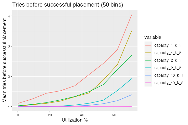
In this simulation, we’re looking at random placement ($k=1$) and best-of-2 ($k=2$), for three values of $c$ and asking how many times we need to go through the iterative best-of-k loop before we get a success. Start with $c = 10$: as we’d expect, best-of-2 outperforms random handily. So much that we never actually have to retry. But for $c = 1$, best-of-2 is only slightly (about 30%) better than random placement. Still better, still useful, but not nearly as super powerful. The third case, $c = 2$ lands somewhere in between.

Next, let’s look directly at how the number of tries varies across a range of $c$ and $k$ values:

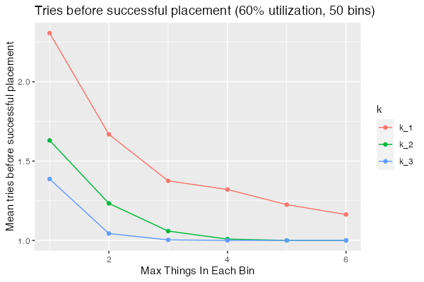
We can see that best-of-2 and best-of-3 outperform random across the range, but even at this modest utilization ($U = 0.6$) they still require significantly more searching for low $c$.

What Can We Learn?

The main lesson here is that, as powerful as best-of-k is, it isn’t magic. A system that needs to find needles in a haystack - those few workers with one free capacity slot - likely needs to use a different approach. The obvious solution is a list of workers with free capacity, but that becomes a scalability and fault tolerance challenge in the distributed setting.

Footnote: Pedantry about Replacement

As we increase $k$ we roll again and again.

Of course, that’s not quite what happens, because in best-of-k we pick the k without replacement (that is the same worker doesn’t appear multiple times in the k we pick). That’s important, because without replacement it means the $k = n$ case succeeds for all $U < 1$, providing us with a nice bound on the behavior as $k$ gets big.

Let’s see what we can learn pulling on that thread a bit.

We’ll try calculate the probability distribution $P(j)$ that our $k$ picks will contain j empty workers. First, there are ${n \choose k}$ ways of picking k from n workers. Then, the number of ways we can pick $j$ non-empty workers from the pool of $(1 - U) n$ non empty-workers is ${n - m \choose j}$. Finally, the number of ways to pick $k - j$ from the non-empty workers is ${m \choose k - j}$. Putting these together, we get:

The case we’re really interested in is the $j = 0$ case where we don’t succeed. I think we can simplify to get:

or, alternatively:

Which provides at least a reasonably useful closed-form way to approximate the per-attempt successes. Our iterative best-of-k algorithm chooses a different k with replacement each time, the mean number of attempts before success becomes:

Now we can re-create the first graph in tidy closed form:

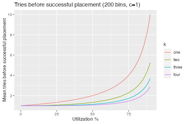
It may be possible to simplify that further, but (as I said above) my combinatorics is super rusty. Take this whole analysis with a big grain of salt.

Other Posts

• 25 Apr 2024 » MemoryDB: Speed, Durability, and Composition.
• 17 Apr 2024 » Formal Methods: Just Good Engineering Practice?
• 04 Mar 2024 » The Builder's Guide to Better Mousetraps