Open and Closed, Omission and Collapse

Were you born in a cave?

This, from Open Versus Closed: A Cautionary Tale by Schroeder et al¹ is one of the most important concepts in systems performance:

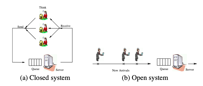
Workload generators may be classified as based on a closed system model, where new job arrivals are only triggered by job completions (followed by think time), or an open system model, where new jobs arrive independently of job completions. In general, system designers pay little attention to whether a workload generator is closed or open.

Or, if you’d prefer it as an image, from the same paper:

While the paper does a good job explaining why it’s so important, I don’t think it even fully justifies what a big difference the open and closed modes of operation have on measurement, benchmarking, and system stability.

Some Examples

Let’s consider a very simple system, along the lines of the one in the image above: a single server, an unbounded queue, and either open or closed customer arrival processes. First, we’ll consider an easy case, where the server latency is exponentially distributed with a mean of 0.1ms. What does the client-observed latency look like for a single-client closed system, closed system with 10 clients, or an open system with a Poisson arrival process?⁶

To answer that question, we need to pick a value for the server utilization ($\rho$), the proportion of the time the server is busy. Here, we consider the case where the server is busy 80% of the time ($\rho = 0.8$)²:

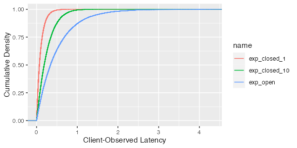
This illustrates one of the principles from the paper:

Principle (i): For a given load, mean response times are significantly lower in closed systems than in open systems.

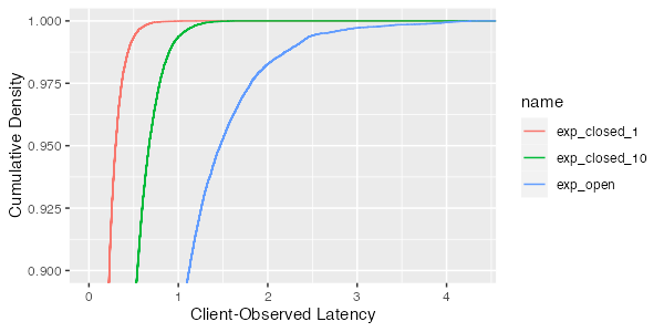
but it also shows us something else: the tail is much longer for the open case than the closed one. We can see more of that if we zoom in on just the tail of the latency distribution (percentiles higher than the 90th):

This difference is even more stark if we consider a server-side distribution with worse behavior. Say, for example, one that with an average response time of 0.1ms 99.9% of the time, and 10ms 0.1% of the time. That’s a bit of an extreme example, but not one that is impossible on an oversubscribed or garbage-collected system, or even one that needs to touch a slow storage device for some requests. What does the response time look like?

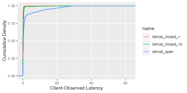
and, zooming in on the tail:

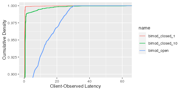
As we would expect, the 99th percentile for the closed system is much lower. For the single-client closed system, where our hypothesis is that the client-observed latency is equal to the server latency because no queue can form, the 99th percentile is below 1ms. For the open system, its over 25ms. This is happening simply because a queue can form. Without a limit on client-side concurrency, the queue grows during the pause, and then must pay down that queue when the long request is over. Sometimes another long response time will happen before the queue drains, stacking latency up further.

Benchmarks and Coordinated Omission

From the results above, you should be able to see that a closed benchmark running against a system which will be open in production could significantly under estimate the tail latency observed by real-world clients (and vice versa). This is a phenomenon that Gil Tene popularized under the name coordinated omission³, which has brought some (but not enough) awareness of it. This isn’t a small or academic point. While our bimodal example is a little extreme, it is not out of the realm of what we see in the real world, and shows that a closed benchmark could underestimate 99th percentile latency by a factor of at least 25.

That mistake is a really easy to make, because the simplest, easiest-to-write, benchmark loop falls into exactly this trap. Here’s a closed-loop benchmark:

while True:
  send request
  wait for response
  write down response time

compare it to an open loop implementation:

while True:
  sleep 1ms
  send request
  (asynchronously write down the response time on completion in a different thread)

The closed loop one is the one I’d probably write if I wasn’t thinking about it. It’s the easiest one to write (at least in a language without nice first-class asynchrony), and the obvious way to approach the problem.

Open Loops, Timeouts, and Congestive Collapse

Coordinated omission and misleading benchmark results aren’t even the most important thing about open loop systems. In my mind, the most important thing to understand is congestive collapse. Probably the simplest version to understand has to do with client behavior, specifically timeouts and retries. The open loop model is optimistic. In the real world of timeouts and retries, its optimistic to believe that jobs arrive independently of job completions. Indeed, even if the underlying arrival rate is Poisson, there is also some additional rate of traffic that arrives due to timeouts.

Let’s go back to our bimodal example from earlier, and look at the queue length over the simulation time for the open and closed cases. As expected, the closed cases drive shorter queues, and the open case’s latency is driven by the queue growing and shrinking as long server-side latency drives short periods where requests are coming in faster than they can be served.

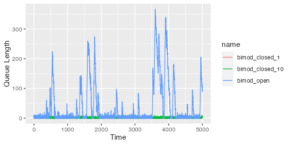
In the long-term, though, because our utilization is only 80% ($\rho = 0.8$), the server always eventually catches up and the queue drains. One way that often happens in production is because of client behavior, specifically retries⁴ after timeouts. What if we take the bimodal system, and make the seemingly very small change of retrying if the response takes longer than 15ms? That seems safe, because it’s still more than 15x the server’s 99th percentile latency. Here’s what our queue length looks like:

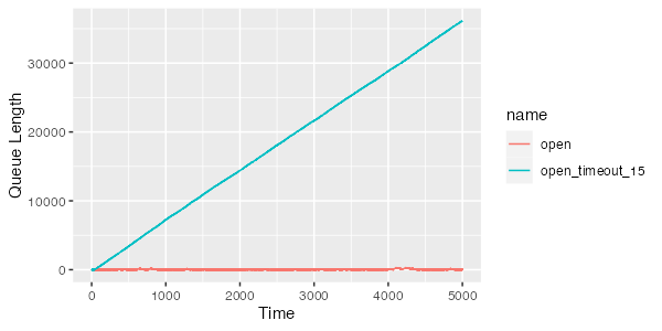
Oh no! Our queue is growing without bound! We have introduced a catastrophe: as soon as the response time exceeds 15ms for a request, we add another request, which slightly increases the arrival rate (increasing $\rho$), which slightly increases latency, which slightly increases the probability that future requests will take more than 15ms, which slightly increases the rate of future retries, and so on to destruction.

Closed systems don’t suffer from this kind of catastrophe, unless they have client behaviors that mistakenly turn them into open systems due to retries. Almost all stable production systems aren’t really open, and instead approximate closed behavior by limiting either concurrency or arrival rate⁵.

Footnotes

1. Despite this being a blog post about a queue theory paper, I’ve tried not to use a lot of queue theory results here, and instead used the results of numerical simulations. I’ve done that for two reasons. One is that I want to make a point about tail latency, and queue theory results around the tail latency of arbitrary distributions aren’t particularly accessible (or, in some cases, don’t exist). Second, a lot of people engage with numerical examples more than they do with theoretical results.
2. For more on the importance of $\rho$ see Latency Sneaks Up on You
3. On Coordinated Omission by Ivan Prisyazhynyy is a good introduction.
4. For a more general look at retry-related problems, and one solution, check out Fixing retries with token buckets and circuit breakers
5. One of the best decisions we made early on in building AWS Lambda was to make concurrency the unit of scaling rather than arrival rate. This makes it significantly easier both for the provider and the customer to avoid congestive collapse behaviors in their systems. The way Lambda uses concurrency is describe in the documentation.
6. These results were generate with a simple simulation. If you would like to check my work, the simulator code that generated these results is available on Github. The code is less than 200 lines of Python, and should be accessible without any knowledge of queue theory.

Other Posts

• 17 Apr 2024 » Formal Methods: Just Good Engineering Practice?
• 25 Mar 2024 » Finding Needles in a Haystack with Best-of-K
• 04 Mar 2024 » The Builder's Guide to Better Mousetraps